Algebra 2 by Richard Wright

Previous LessonTable of Contents Next Lesson

Are you not my student and
has this helped you?

0-08 Draw Scatter Plots and Best-Fitting Lines

Experiments and studies that investigate relationships such as time a person spends reading the Bible and how well the person treats others sometimes give a linear relationship. In this proposed study, the more time spent reading the Bible may cause the person to treat others better.

Scatter Plot

A scatter plot is a graph of many data points. They help identify trends in the data by using correlation coefficient, r. The correlation coefficient is a number between –1 and 1 that measure how well the data fits a line. Positive correlation coefficients are for positive slopes, and negative coefficients for negative slopes. The better the points fit a line, the closer the correlation coefficient will be to 1 or –1.

Positive correlation means the slope of the scatter plot tends to be positive. The correlation coefficient will be positive.

Negative correlation means the slope of the scatter plot tends to be negative with a negative correlation coefficient.

No correlation means there is no obvious pattern from the scatter plot. The correlation coefficient will be near zero.

Example 1

For each scatter plot, a) tell whether the data have a positive correlation, a negative correlation, or approximately no correlation, and b) tell whether the correlation coefficient is closest to –1, –0.5, 0, 0.5, or 1.

Solution

Graph I: The points are nearly in a straight line with a positive slope so positive correlation with r ≈ 1.

Graph II: The points resemble a line with negative slope, but the points are not perfectly in a line so negative correlation with r ≈ −0.5.

Graph III: The points do not appear to make a line, so no correlation with r ≈ 0.

Best-fitting line

The best-fitting line is the line that most closely approximates the data in a scatter plot.

Find Best-Fitting Lines Using a Graphing Utility

While estimating a best-fitting line works reasonably well, there are better statistical techniques for minimizing the distances from line to the data points. One such technique is called least squares regression and can be computed by many graphing calculators, spreadsheet software, statistical software, and many web-based calculators. Least squares regression is one means to determine the best-fitting for the data. Least squares regression is often called linear regression.

Finding Linear Regression on a TI-84

1. Push STAT and select Edit….
2. Enter the x-values in List 1 (L1) and the y-values in List 2 (L2).
3. To see the graph of the points
   1. Push Y= and clear any equations.
   2. While still in Y=, go up and highlight Plot1 and press ENTER.
   3. Press ZOOM and select ZoomStat.
4. Push STAT and move over to the CALC menu.
5. Select LinReg(ax+b) (Linear Regression).
6. Make sure the Xlist: is L1,the Ylist: is L1, the FreqList: is blank, and the Store RegEQ: is Y1.
   1. Get Y1 by pressing VARS and select Y-VARS menu.
   2. Select Function….
   3. Select Y1.
7. Press Calculate

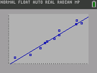
The calculator will display the equation. To see the graph of the points and line, press GRAPH.

Note: Older TI graphing calculators do not have the screen in steps 6 and 7. After selecting the LinReg(ax+b), the screen just shows "LinReg(ax+b)". Press ENTER again to see the result. To see the graph, enter the equation into the Y= screen and press GRAPH.

Finding Linear Regression on a NumWorks graphing calculator

1. On the home screen select Regression.
2. In the Data tab, enter the points.
3. Move to the Graph tab.
4. The default is a linear regression and is displayed at the bottom of the screen. To change the regression type
   1. Press OK.
   2. Select Regression.
   3. Select the desired regression type.

Example 4: Finding a Least Squares Regression Line

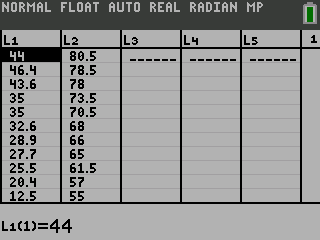
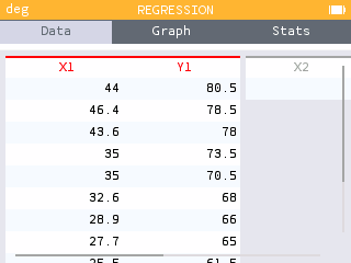
Find the least squares regression line using the cricket-chirp data in Table 1.

Solution (TI-84)

On a TI-84 graphing calculator

1. Push STAT and select Edit….
2. Enter the input x-values (chirps) in List 1 (L1).
3. Enter the output y-values (temperature) in List 2 (L2).
   

   

4. Press STAT and move over to the CALC menu. Then select Linear Regression LinReg(ax+b).
5. Make sure the Xlist: is L1, the Ylist: is L2, and press Calculate.
   

   Note: To see the graph, enter Y1 for Store RegEQ: before pressing Calculate. Y1 is found in VARS → Y-VARS ↓ Function… ↓ Y1

   
   

   

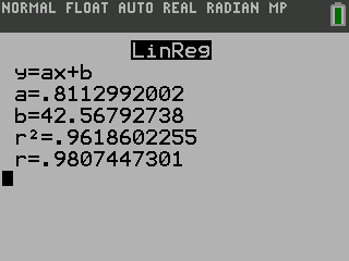
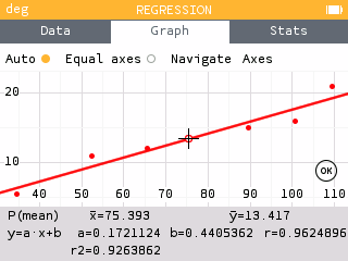
T(c) = 0.811c + 42.57

The graph of the scatter plot with the least squares regression line is shown in figure 11.

Solution (NumWorks)

On a NumWorks graphing calculator

1. Select Regression from the home screen.
2. Go to the Data tab.
3. Enter the input x-values (chirps) in the first list (X1).
4. Enter the output y-values (temperature) in the second list (Y1).
   

   

5. Go to the Graph tab.
6. The default is linear regression and the equation is at the bottom of the screen. If needed, change the regression type by pressing OK and choosing a different regression type.

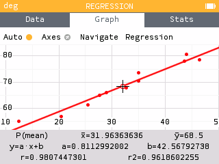
T(c) = 0.811c + 42.57

Practice Problems (*Optional)

For each scatter plot, a) tell whether the data have a positive correlation, a negative correlation, or approximately no correlation, and b) tell whether the correlation coefficient is closest to −1, −0.5, 0, 0.5, or 1.

1. 
2. 
3. 
4. 

a) Draw a scatter plot using the data in the table, then b) tell whether the data have a positive correlation, a negative correlation, or approximately no correlation, and c) tell whether the correlation coefficient is closest to −1, −0.5, 0, 0.5, or 1.

5. x	0	1	2	3	4	5
   y	5	4.2	4.3	3.5	3.1	2.3

6. *

   x	0.5	1	1.5	2	2.5	3	3.5	4
   y	2	2.2	2.4	2.6	2.8	3	3.2	3.4

a) Draw a scatter plot using the data in the table, then b) write the equation of the best fitting line.

7. x	0	0.5	1	1.5	2	2.5	3	3.5	4
   y	1	1.6	2	2.4	3	3.6	4	4.4	5

8. x	0	0.5	1	1.5	2	2.5	3	3.5	4
   y	5	4.4	3.8	3.2	2.6	2	1.4	0.8	0.2

9. x	0	0.5	1	1.5	2	2.5	3	3.5	4
   y	2.1	2.3	2.5	2.7	2.9	3.1	3.3	3.5	3.7

10. *

    x	0	0.5	1	1.5	2	2.5	3	3.5	4
    y	5.8	5	4.2	3	1.8	1	0.2	−1	−2

Problem Solving

11. In a physics lab, Sarah is investigating the relationship between position, velocity, and time. She recorded her data of time, t in seconds, and position, x in meters, in the following table. a) Draw a scatter plot of her data and b) write the equation of the best fitting line. Use t for time and x for position. The slope is the velocity of the moving object.
    

    t	0.05	0.10	0.15	0.20	0.25	0.30	0.35
    x	0.05	0.10	0.16	0.22	0.27	0.33	0.37

12. 

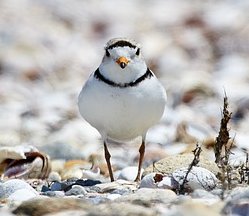
    Piping Plovers are small birds that live on sandy beaches in the United States. In 1985 they were put on the endangered species list. The following table gives the number of breeding pairs found on the Atlantic Coast. a) Draw a scatter plot of the data and b) write the equation of the best fitting line. Use P for Plovers and t for years since 1985.

    t	1	3	5	7	9	11	13	15	17	19	21	23	25
    P	790	886	982	1013	1162	1364	1379	1437	1690	1658	1749	1849	1782

Mixed Review

13. *(0-07) Graph y ≤ |x + 1| − 3.
14. (0-07) Graph \(y > \frac{2}{3} x-1\).
15. (0-06) a) Describe the transformation, then b) graph the absolute value function. y = −|x − 2| + 1
16. *(0-05) Graph \(y = -\frac{3}{2} x + 2\).
17. *(0-04) Write the equation of the line passing through (−2, 1) and (3, 4).
18. (0-03) Solve |3x − 5| = 13.
19. (0-02) a) Read 1 Kings 7:13. When King Solomon was building the temple, who did he hire for making the bronze things? b) Read 1 Kings 7:23. What was the circumference of the water vessel called “The Sea”? Give the answer in cubits. c) Use the internet to convert the answer from part b into feet. d) Using the answer from part c, what was the radius of The Sea in feet?
20. (0-01) Solve for y. 3x + 5y = 15

Answers

1. Negative correlation; r ≈ −1
2. No correlation; r ≈ 0
3. Positive correlation; r ≈ 0.5
4. Positive correlation; r ≈ 1
5. ; negative correlation; r ≈ −0.5
6. ; positive correlation; r ≈ 1
7. 
8. 
9. 
10. 
11. 
12. 
13. 
14. 
15. Reflected over the x-axis, moved 2 right and 1 up;
16. 
17. \(y=\frac{3}{5}x+\frac{11}{5}\)
18. \(-\frac{8}{3}\), 6
19. c) 45 feet, d) 7.16 ft
20. \(y=-\frac{3}{5}x+3\)