
Algebra 2 by Richard Wright
Are you not my student and
has this helped you?
Objectives:
SDA NAD Content Standards (2018): AII.5.1, AII.5.2, AII.6.5, AII.7.1, AII.7.2
Equations that model real life situations do not just magically appear out of thin air. In real life situations, people need to collect data which can plotted as points on a graph. Mathematical modeling turns those points into a function that models that situation.
Mathematical modeling is the process of finding a function that best fits the given points or data.
In lesson 2-02, instructions were given to find a quadratic model given the x-intercepts and another point. The same idea can be used to write general polynomial models given the x-intercepts and one other point.
Write a polynomial model with x-intercepts (−2, 0), (1, 0), and (5, 0) and passes through (2, 4).
Solution
There are three x-intercepts so write the general polynomial with three factors.
y = a(x – k1)(x – k2)(x – k3)
Substitute the x-intercepts for the k's.
y = a(x – (–2))(x – 1)(x – 5)
y = a(x + 2)(x – 1)(x – 5)
Substitute the other point for x and y.
4 = a(2 + 4)(2 – 1)(2 – 5)
4 = a(–18)
$$ -\frac{2}{9}=a $$
Finally, write the function by substituting the x-intercepts and a into the general polynomial model.
$$ y=-\frac{2}{9}\left(x+4\right)\left(x-1\right)\left(x-5\right) $$
If none of the special points, vertex or x-intercepts are given, then the process is a little longer. The first step is to determine the degree of the function. If the function is to through all the points, then the process of finding finite differences will show the degree.
To find the degree of a function using finite differences,
Find the degree of the polynomial function passing through (0, −4), (1, −4), (2, −2), (3, 8), (4, 32), (5, 76), (6, 146).
Solution
Write the points as a table.
| x | 0 | 1 | 2 | 3 | 4 | 5 | 6 |
|---|---|---|---|---|---|---|---|
| y | −4 | −4 | −2 | 8 | 32 | 76 | 146 |
Subtract the y-values.
| x | 0 | 1 | 2 | 3 | 4 | 5 | 6 | ||||||||||||||||||
|---|---|---|---|---|---|---|---|---|---|---|---|---|---|---|---|---|---|---|---|---|---|---|---|---|---|
| y | −4 | −4 | −2 | 8 | 32 | 76 | 146 | ||||||||||||||||||
| \ | / | \ | / | \ | / | \ | / | \ | / | \ | / | ||||||||||||||
| 0 | 2 | 10 | 24 | 44 | 70 |
Subtract those differences.
| x | 0 | 1 | 2 | 3 | 4 | 5 | 6 | ||||||||||||||||||
|---|---|---|---|---|---|---|---|---|---|---|---|---|---|---|---|---|---|---|---|---|---|---|---|---|---|
| y | −4 | −4 | −2 | 8 | 32 | 76 | 146 | ||||||||||||||||||
| \ | / | \ | / | \ | / | \ | / | \ | / | \ | / | ||||||||||||||
| 0 | 2 | 10 | 24 | 44 | 70 | ||||||||||||||||||||
| \ | / | \ | / | \ | / | \ | / | \ | / | ||||||||||||||||
| 2 | 8 | 14 | 20 | 46 |
Subtract those differences.
| x | 0 | 1 | 2 | 3 | 4 | 5 | 6 | ||||||||||||||||||
|---|---|---|---|---|---|---|---|---|---|---|---|---|---|---|---|---|---|---|---|---|---|---|---|---|---|
| y | −4 | −4 | −2 | 8 | 32 | 76 | 146 | ||||||||||||||||||
| \ | / | \ | / | \ | / | \ | / | \ | / | \ | / | ||||||||||||||
| 0 | 2 | 10 | 24 | 44 | 70 | ||||||||||||||||||||
| \ | / | \ | / | \ | / | \ | / | \ | / | ||||||||||||||||
| 2 | 8 | 14 | 20 | 46 | |||||||||||||||||||||
| \ | / | \ | / | \ | / | \ | / | ||||||||||||||||||
| 6 | 6 | 6 | 6 |
These differences are all the same. It took three levels of subtracting for the differences to be constant, so the degree of the function is 3.
To find a polynomial function that passes through given points,
Method 1: Solve a System of Equations by Hand (This lesson uses Method 2)
Method 2: Use a Regression on a Graphing Calculator
Note: Older TI graphing calculators do not have the screen in steps 6 and 7. After selecting the LinReg(ax+b), the screen just shows "LinReg(ax+b)". Press ENTER again to see the result. To see the graph, enter the equation into the Y= screen and press GRAPH.
Find the polynomial function passing through the (0, −4), (1, −4), (2, −2), (3, 8), (4, 32), (5, 76), (6, 146).
Solution
These are the same points as example 2, so the degree is 3. This example will illustrate method 2: using a graphing calculator to do a regression.
| TI-84 | NumWorks |
|---|---|
|
Push STAT and select Edit… Enter the x-values in List 1 (L1) and the y-values in List 2 (L2). 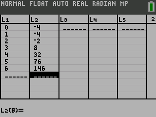
Push STAT and move over to the CALC menu. Select the type of regression. Make sure the Xlist: is L1, the Ylist: is L1, the FreqList: is blank, and the Store RegEQ: is Y1. Get Y1 by pressing VARS and select Y-VARS menu. Select Function…. Select Y1. 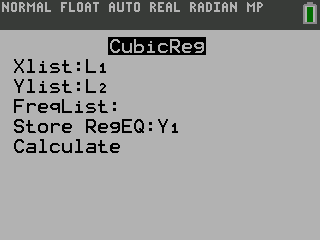
Press Calculate 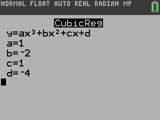
|
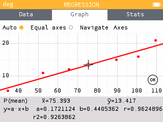
On the home screen select Regression. In the Data tab, enter the points. 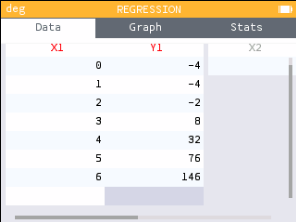
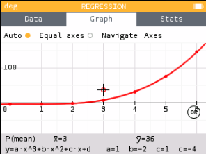
Move to the Graph tab. The default is a linear regression and is displayed at the bottom of the screen. To change the regression type
|
| Both calculators say that a = 1, b = −2, c = 1, and d = −4. Substitute those into the general polynomial function given on the calculator. The polynomial function through those points is y = x3 − 2x2 + x − 4. | |
Find the polynomial function through (0, −16), (1, −10.5), (2, −4), (3, 3.5), (4, 12), (5, 21.5), (6, 32).
Solution
Because these are not special points, use finite differences to find the degree.
| x | 0 | 1 | 2 | 3 | 4 | 5 | 6 | ||||||||||||||||||
|---|---|---|---|---|---|---|---|---|---|---|---|---|---|---|---|---|---|---|---|---|---|---|---|---|---|
| y | −16 | −10.5 | −4 | 3.5 | 12 | 21.5 | 32 | ||||||||||||||||||
| \ | / | \ | / | \ | / | \ | / | \ | / | \ | / | ||||||||||||||
| 5.5 | 6.5 | 7.5 | 8.5 | 9.5 | 10.5 | ||||||||||||||||||||
| \ | / | \ | / | \ | / | \ | / | \ | / | ||||||||||||||||
| 1 | 1 | 1 | 1 | 1 |
There were two levels of finite differences, so the degree is 2 so it is quadratic.
Use technology to find the quadratic function.
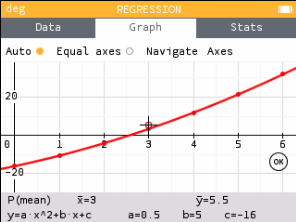
The polynomial function through the points is y = 0.5x2 + 5x − 16.
Finite differences do not work to find the degree of the polynomial for data measured many experiments or studies. This is because many situations do not have an exact model, just an approximation. These situations use a regression which is a calculated best-fitting model.
To find the best-fitting polynomial model using a graphing calculator, use method 2 from above. It may be necessary to try a couple different degrees to find the best fit. For example, the cubic may be close, but the quartic might be closer.
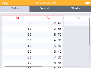
Find the best-fitting polynomial model for the population of Michigan given in the table. Then estimate the population in 2050.
| Year | 1900 | 1910 | 1920 | 1930 | 1940 | 1950 | 1960 | 1970 | 1980 | 1990 | 2000 | 2010 |
|---|---|---|---|---|---|---|---|---|---|---|---|---|
| Population (millions) | 2.42 | 2.83 | 3.72 | 4.83 | 5.32 | 6.41 | 7.83 | 8.88 | 9.21 | 9.31 | 9.92 | 9.93 |
Use the number of years after 1900 as the x-coordinate. It is usually called t for time. The population is y. Notice population is in millions.
Enter the data in the STAT or Regression table.
Try several regressions to see which is best.
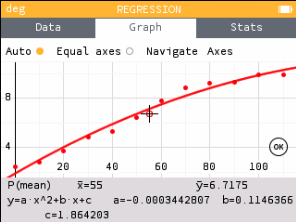
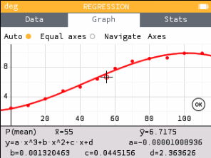
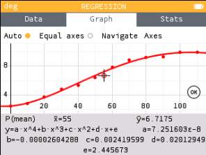
Notice that the cubic seems to fit better than the quadratic. Also notice that the quartic and cubic look almost identical. When that happens use the lower degree. Thus, this situation should use the cubic model.
y = −0.0000101x3 + 0.00132x2 + 0.0445x + 2.364
Substitute more meaningful variables for x and y. Use t for x and P for y.
P = −0.0000101t3 + 0.00132t2 + 0.0445t + 2.364
To estimate the population in 2050, substitute t = 150.
P = −0.0000101(150)3 + 0.00132(150)2 + 0.0445(150) + 2.364
P = 4.65
The population would be 4.65 million if this trend continues. Since this is half of the population in 2000 and 2010 and population tends to grow over long periods of time, this model is likely not valid for 2050.
217 #1, 3, 5, 7, 9, 11, 13, 14, 17, 19, Mixed Review = 15
Mixed Review

 ; (−1, 0), (1, 0), (3, 0)