The test statistics used in conjunction with the
normal and Student t distributions assume
certain parameters about the parent populations,
specifically, normality and variance homogeneity.
Quite often in behavioral science research such
restrictive assumptions cannot be made and certain
nonparametric tests have been developed which
help us analyze such data.
A common distribution encountered in such nonparametric tests
is the ![]() 2 distribution.
2 distribution.
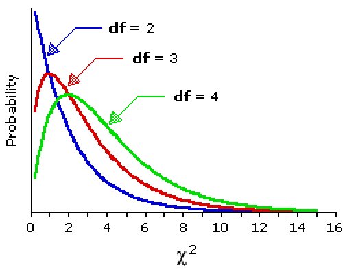
The ![]() 2
family of distributions is
characterized by one parameter called the degrees of freedom which is
often denoted by v (the greek letter nu) and used as a subscript:
2
family of distributions is
characterized by one parameter called the degrees of freedom which is
often denoted by v (the greek letter nu) and used as a subscript:
![]() 2v.
2v.
Gosset
first described the distribution of s2.
It is related to the ![]() 2
by the simple factor (n-1)/
2
by the simple factor (n-1)/ 2.
Although he wasn't able to prove this mathematically, he
demonstrated it by dividing a prison population of 3000 into
750 random samples of size four and used their heights.
2.
Although he wasn't able to prove this mathematically, he
demonstrated it by dividing a prison population of 3000 into
750 random samples of size four and used their heights.
A common application of the ![]() 2 distribution
is in the comparison of expected with observed
frequencies. When there is but one nominal variable,
this is often termed goodness of fit.
In this case we are testing whether or not the
observed frequencies are within statistical
fluctuations of the expected frequencies.
Although one typically checks for high
2 distribution
is in the comparison of expected with observed
frequencies. When there is but one nominal variable,
this is often termed goodness of fit.
In this case we are testing whether or not the
observed frequencies are within statistical
fluctuations of the expected frequencies.
Although one typically checks for high
![]() 2
values, the second example below illustrates the
possible significance of a low
2
values, the second example below illustrates the
possible significance of a low
![]() 2 value.
2 value.
Example: On July 14, 2005 we collected 10 trials of 20 pennies each where these 20 pennies were set on edge and the table banged. We observed 145 heads. We can compare the observed with expected frequencies and test for goodness of fit as shown in the table below. There is but one degree of freedom since the number of tails is dependent on the number of heads (200 - 145 = 55).
| Side: | Head | Tail |
|---|---|---|
| Observed | 145 | 55 |
| Expected | 100 | 100 |
| (Obs-Exp) | 45 | -45 |
| (O-E)2 | 2045 | 2045 |
| (O-E)2/E | 20.45 | 20.45 |
Solution:
We form the ![]() 2
statistic by summing the
(O-E)2/E and get 2045/100 + 2045/100 = 40.9.
We can then compare this
2
statistic by summing the
(O-E)2/E and get 2045/100 + 2045/100 = 40.9.
We can then compare this
![]() 2 with critical
2 with critical
![]() 2
values or find an associated P-value. The critical
2
values or find an associated P-value. The critical
![]() 2
value for df=1 and one-tailed, alpha=0.05 is 3.841.
Our results are far to the right of 3.841
so are VERY significant (P-value=1.6×10⁻¹⁰).
A table of critical
2
value for df=1 and one-tailed, alpha=0.05 is 3.841.
Our results are far to the right of 3.841
so are VERY significant (P-value=1.6×10⁻¹⁰).
A table of critical
![]() 2
values for select values is given below.
2
values for select values is given below.
| df\upper tail area | 0.99 | 0.95 | 0.90 | 0.10 | 0.05 | 0.01 |
|---|---|---|---|---|---|---|
| 1 | 0.00016 | 0.0039 | 0.016 | 2.706 | 3.841 | 6.635 |
| 2 | 0.020 | 0.103 | 0.211 | 4.605 | 5.991 | 9.210 |
| 3 | 0.115 | 0.352 | 0.584 | 6.251 | 7.815 | 11.34 |
| 4 | 0.297 | 0.711 | 1.064 | 7.779 | 9.488 | 13.28 |
| 5 | 0.554 | 1.145 | 1.610 | 9.236 | 11.07 | 15.09 |
| 10 | 2.558 | 3.940 | 4.865 | 15.99 | 18.31 | 23.21 |
| 15 | 5.229 | 7.261 | 8.547 | 22.31 | 25.00 | 30.58 |
| 20 | 8.260 | 10.85 | 12.44 | 28.41 | 31.41 | 37.57 |
| 25 | 11.52 | 14.61 | 16.47 | 34.38 | 37.65 | 44.31 |
| df > 30: use z = sqrt(2chi2)-sqrt(2df-1) | ||||||
Example: On July 12, 2005 we collected 192 dice rolls, each person present using a different die and each person doing 24 rolls. Were the results within the expected range?
| Pips: | 1 | 2 | 3 | 4 | 5 | 6 |
|---|---|---|---|---|---|---|
| Observed | 27 | 23 | 30 | 35 | 40 | 37 |
| Expected | 32 | 32 | 32 | 32 | 32 | 32 |
| (Obs-Exp) | -5 | -9 | -2 | 3 | 8 | 5 |
| (O-E)2 | 25 | 81 | 4 | 9 | 64 | 25 |
| (O-E)2/E | 0.78125 | 2.53125 | 0.125 | 0.28125 | 2.00 | 0.78125 |
Solution:
We form the ![]() 2
statistic by summing the (O-E)2/E
and get 208/32=6.5. We can then compare this
2
statistic by summing the (O-E)2/E
and get 208/32=6.5. We can then compare this
![]() 2
with a critical
2
with a critical ![]() 2.
Only if it is more extreme is it worth finding a P-value.
We have 6 - 1 = 5 degrees of freedom.
The critical
2.
Only if it is more extreme is it worth finding a P-value.
We have 6 - 1 = 5 degrees of freedom.
The critical ![]() 2 values for df=5,
two-tailed, and alpha=0.10 are 1.145 and 11.07.
Since our
2 values for df=5,
two-tailed, and alpha=0.10 are 1.145 and 11.07.
Since our ![]() 2 is within this range,
our results are within the range we can expect to occur by chance.
Notice the lower
2 is within this range,
our results are within the range we can expect to occur by chance.
Notice the lower ![]() 2
cut off. When people fabricate a random
distribution they are likely to make it too uniform and
get too small of a
2
cut off. When people fabricate a random
distribution they are likely to make it too uniform and
get too small of a ![]() 2 which can be checked as above,
but the
2 which can be checked as above,
but the ![]() 2 would likely be less than 1.145.
Working backwards we see the sum of the (O-E)2
would have to be less than 36 so if one were 5 or less away
and the rest much closer, we might wonder.
2 would likely be less than 1.145.
Working backwards we see the sum of the (O-E)2
would have to be less than 36 so if one were 5 or less away
and the rest much closer, we might wonder.
As noted at the bottom of the table above,
when the degrees of freedom are large,
a z-score can be formed and compared
against a standard normal distribution.
Note also that the mean of any ![]() 2 is the
degrees of freedom. This might be helpful
to realize where the distribution is centered.
2 is the
degrees of freedom. This might be helpful
to realize where the distribution is centered.
The ![]() 2
goodness of fit does not indicate
what specifically is signficant. To find that out
one must calculate the standardized residuals.
The standardized residual is the signed square root
of each category's contribution to the
2
goodness of fit does not indicate
what specifically is signficant. To find that out
one must calculate the standardized residuals.
The standardized residual is the signed square root
of each category's contribution to the
![]() 2 or
R = (O - E)/sqrt(E).
When a standardized residual has a magnitude
greater than 2.00, the corresponding category is
considered a major contributor to the significance.
(It might be just as easy to see which (O - E)2/E
entries are larger than 4, but standardized residuals are typically
provided by software packages.)
2 or
R = (O - E)/sqrt(E).
When a standardized residual has a magnitude
greater than 2.00, the corresponding category is
considered a major contributor to the significance.
(It might be just as easy to see which (O - E)2/E
entries are larger than 4, but standardized residuals are typically
provided by software packages.)
There are potential problems associated with small expected frequencies in contingency tables. Historically, when any cell of a 2×2 table was less than 5 a Yates' correction of continuity was advised. However, it has been shown that this can result in a loss of power (a tendancy not to reject a false null hypothesis). Care should be exercised and advise sought. Larger contingency tables can also be problematic when more than 20% of the cells have expected frequencies less than 5 of if there are any cells with 0. One solution is to combine adjacent rows or columns, but only if it makes sense.
The McNemar test is a
![]() 2 test for
matched pair (like pre-/post-test) treatment designs.
In the 2×2 contingency table, the A and
D cells contain the change responses and the
B and C cells contain the no change responses.
The
2 test for
matched pair (like pre-/post-test) treatment designs.
In the 2×2 contingency table, the A and
D cells contain the change responses and the
B and C cells contain the no change responses.
The ![]() 2
simplifies to (A - D)2/(A + D)
and is interpretted as per usual (with df = 1).
2
simplifies to (A - D)2/(A + D)
and is interpretted as per usual (with df = 1).
The Stuart-Maxwell test extends the McNemar test to
3×3 contingency tables. Here the no change situation
occupies the main diagonal (upper left to lower right) and we form
the ![]() 2
from averaged pairs of differences
weighted by the square of the differences between
the other row/column totals. We leave the curious
reader to a software package or statistics textbook
for the actual formula.
2
from averaged pairs of differences
weighted by the square of the differences between
the other row/column totals. We leave the curious
reader to a software package or statistics textbook
for the actual formula.
Remember, the prior lesson
referred to the Pearson contingency coefficient (C)
and Cramer's V coefficient which are defined in
terms of the ![]() 2
statistic. Specifically,
C = sqrt(chi2/(n + chi2)) and
V = sqrt(chi2/(n(q -1 )),
where q is the smaller of the number of rows or columns
in the contingency table.
2
statistic. Specifically,
C = sqrt(chi2/(n + chi2)) and
V = sqrt(chi2/(n(q -1 )),
where q is the smaller of the number of rows or columns
in the contingency table.
In closing we should note the importance of focusing on a
small number of well-conceived hypotheses in research rather
than blindly calculating a bevy of
![]() 2 statistics for
all variable pairs and ending up with 5% of your results
being significant at the 0.05 level!
You would even expect 1% of your results,
due to pure random chance in your sample selection,
to be significant at the 0.01 level.
Since there are n(n - 1)/2 possible pairings
for n variables, one would have 5050 pairs for
100 variables of which over 250 could look significant
at the 0.05 level. Beware!
2 statistics for
all variable pairs and ending up with 5% of your results
being significant at the 0.05 level!
You would even expect 1% of your results,
due to pure random chance in your sample selection,
to be significant at the 0.01 level.
Since there are n(n - 1)/2 possible pairings
for n variables, one would have 5050 pairs for
100 variables of which over 250 could look significant
at the 0.05 level. Beware!
| BACK | HOMEWORK | ACTIVITY | CONTINUE |
|---|