Lab 11: Measuring Atomic Decay and Modeling Decay Using Dice
Archie Wheeler
Arnold Chand
04.09.2012
A pdf version of this lab may downloaded here.
The doc version of this lab may be downloaded here.
Abstract
This lab's purpose was to test the exponential law of decay of a radioactive source and to measure the half-lives and decay constants of indium, silver, and 6-sided dice (some groups used 12-sided). Two of the three parts of our lab successfully proved the model we were attempting to confirm, and the one part that failed to support the model only failed because of a lab blunder on our part. Due to the very unstable nature of some silver nuclei, much of the silver had already decayed before we were able to measure it.
Aside from that blunder, our lab was relatively free from systematic error. Much of the error that we experienced was due to confounding background radiation and the stochastic nature of atomic decay.
Contents
Objectives
- To test the exponential law of decay of a radioactive source, and to measure the half-lives and the decay constants of neutron activated silver and indium.
Setup
Materials:- GM tube in stand
- Indium (In155 95.7%, In113 4.3%)
- Silver (Ag10751.83%, Ag10948.17%)
- Pasco Signal Interface II, Science Workshop and Graphical Analysis software
- Graphical Analysis software
Methods
Part 1. Determination of the Half-life of Indium 116
Using the Pasco GM tube, we measured the background radiation of the lab. We set the sample rate for 30 seconds with non radiation source near the Geiger counter and counted the background radiation for 30 seconds. We then obtained an indium sample and placed it under the Geiger counter for 60 minutes.
During this time, we completed part 3 of the lab.
The series expansion of e-λ can be shown through a Taylor polynomial. At t=0, the value is 1. At t=0, the first derivative can be shown to be -λ, at t=0, the second derivative is shown to be λ2, and so forth. Thus the expansion is 1-(λt)/1!+(λt)2/2!+...+(-1)n(λt)n/n!+...
At small intervals of λt, a linear approximation can be used. So we created a graph of the first five minutes and calculated λ from the slope.
After we obtained an hour's worth of data, we we did an exponential fit of C=C0e-λt+BC, and calculated the value of C0 and λ. Using λ, we calculated the half-life τ and compared it to the accepted value of 54.0 minutes.
Part 2. Determination of the Half-lives of Ag 108 and Ag 110
Using a similar setup to part one, we set the sampling options to be 5 seconds and the stop time to 420 seconds. We brought the radioactive silver from the howitzer and placed it in the tray at the highest position. We then allowed the Geiger counter to record events for 420s. Ag108 has a half-life τ of 2.4 minutes, while Ag110 has a half-life τ of 24seconds. Thus, the decay of the Ag110 will be dominant over the first 100 seconds, and the decay of the Ag108 will be dominant after the first 150 seconds. We can fit exponential decay lines to both of these regions to find out the half-lives of each of these isotopes.
Part 3. Simulation of Radioactive Decay Using Dice.
Dice can be used to model radioactive decay. If we assume that any given die has a one-in-six chance of decaying in a given iteration, we can roll a certain sample of dice, and remove all the die that show a one and have the remaining sample for the next iteration.
We started with 100 dice and performed about 15 iterations until we had observed three half-lives. We used Graphical Analysis and made a graph of N vs. the trial number for both our results and the results of the class, and compared our results to the expected values of τ=6ln(2)=4.16 trials.
Data and Analysis
Part 1. Determination of the Half-life of Indium 116
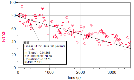
A linear fit of the first 500 seconds of a Geiger count vs. time graph.
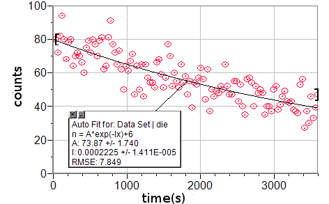
An exponential decay fit of 3600 seconds of a Geiger count vs. time graph.
Results:
Background radiation: 6 events per 30 seconds
τaccepted=54.0min
λlinear=slope/y-intercept=.0001734s-1
τlinear=ln(2)/λ=3995s=66.60min
%Errorlinear=23.33%
λexponential=0.0002225s-1
τexponential=3115s=51.92min
%Errorexponential=3.84%
The series expansion approximation proved to be much more inaccurate than we would have liked it to be, but this is because there is a very large amount of error inherent in the setup. At 1 sample per 30 seconds over a span of 300 second, this only gave us 10 samples. Also, due to the random nature of decaying particles, even if our setup were perfect, we would actually be very surprised if the particles decayed in a very straight line.
But this percent error diminished as we took more samples into consideration over a longer period of time with an exponential decay model. If we had wanted to be much more rigorous in this part of the experiment, we would have taken a longer amount of time to calibrate our experiment to the background radiation (as opposed to our measly one-significant-figure accuracy).
Part 2. Determination of the Half-lives of Ag 108 and Ag 110
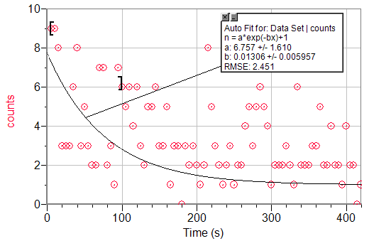
An exponential decay fit to the first 100 seconds of a Geiger count vs. time graph.
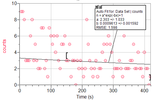 An exponential decay fit to t>150s of a Geiger count vs. time graph of Ag.
Background radiation: 1 event per 5 seconds
τAg110-accepted=24s
τAg108-accepted=2.4min=144s
λAg108=6.757s-1
τAg108=.102s
%Error = 99.9993%
λAg110=2.303s-1
τAg108=.3009s-1
%Error = 98.74%
These errors were disgusting, but I believe that I know at least part of the problem. When we were beginning the lab, I quickly ran to get the silver without first setting up the experiment. I got the silver and then returned to the workstation to calibrate the Geiger counter to the background conditions and setup the sampling settings. By the time I was finished, perhaps three to five minutes had passed, and the silver had already decayed so much that silver's radiation could not be effectively distinguished from the random background radiation.
I had wanted to do this part of the lab over again, but there was no silver that was sufficiently heated to get more data for this part.
Part 3. Simulation of Radioactive Decay Using Dice.
Our data
| trials | dice |
|---|---|
| 0 | 100 |
| 1 | 82 |
| 2 | 75 |
| 3 | 64 |
| 4 | 52 |
| 5 | 50 |
| 6 | 44 |
| 7 | 38 |
| 8 | 34 |
| 9 | 30 |
| 10 | 20 |
| 11 | 16 |
| 12 | 15 |
| 13 | 11 |
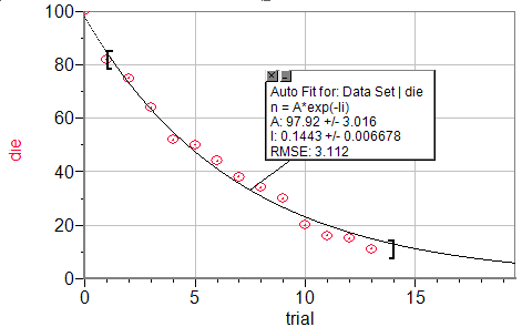
Our graph of number of die after trials
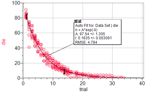
Class graph of number of die after trials
Expected Results:
λ = 1/6
N0=100
Our data:
λ = 0.1443
%Error = 13.42%
N0=97.92
%Error = 2.08%
Class data:
λ = 0.1635
%Error = 1.896%
N0=97.54
%Error = 2.46%
I really do not see any source for error in this part except for the inherent statistical error that will arise in any experiment involving randomness. This error could be reduced by increasing the number of runs or by starting with more dice, however, this error will never go away completely.
Conclusion
I believe that at least two parts of this lab were successes. In both the first and third parts of this lab, we were able to obtain results that matched fairly well with our the accepted models. It is comforting to know that some of this error is completely outside of our control, as there exists an uncontrollable randomness in atomic decay. (Too bad too, because this is the same uncontrollable randomness that means that I can't make a living off of gambling.)
We ran into some major problems in the second part of our experiment, in that we waited too long before we took data. The silver 110 had already undergone many half-lives and the silver 108 several half-lives before we even began to measure them with the Geiger counter.
Yet, the principles that we were trying to measure seemed to hold up well to experimental examination, and at the end of the day, that is what really counts. If we wanted to obtain more accuracy with the indium, we would have had to eliminate as much background radiation as possible and increased the amount of indium in our sample. To make the silver experiment more accurate, we should have eliminated as much background radiation as possible and perhaps moved our lab closer to the Howitzer. To decrease the inherent error in the dice, we should have probably run several computer simulations with millions of dice.
Signature
Archie Wheeler
03.26.12