Precalculus by Richard Wright
Has this helped you?
This book is available
in print and ebook.

Precalculus by Richard Wright
Has this helped you?
This book is available
in print and ebook.
Jesus answered, “It is written: ‘Man shall not live on bread alone, but on every word that comes from the mouth of God.’” Matthew 4:4 NIV
Summary: In this section, you will:
SDA NAD Content Standards (2018): PC.5.4, PC.6.6, PC.7.1, PC.7.2, PC.7.3
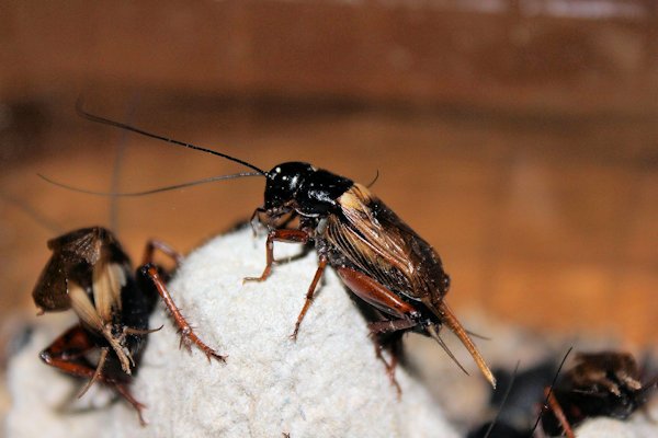
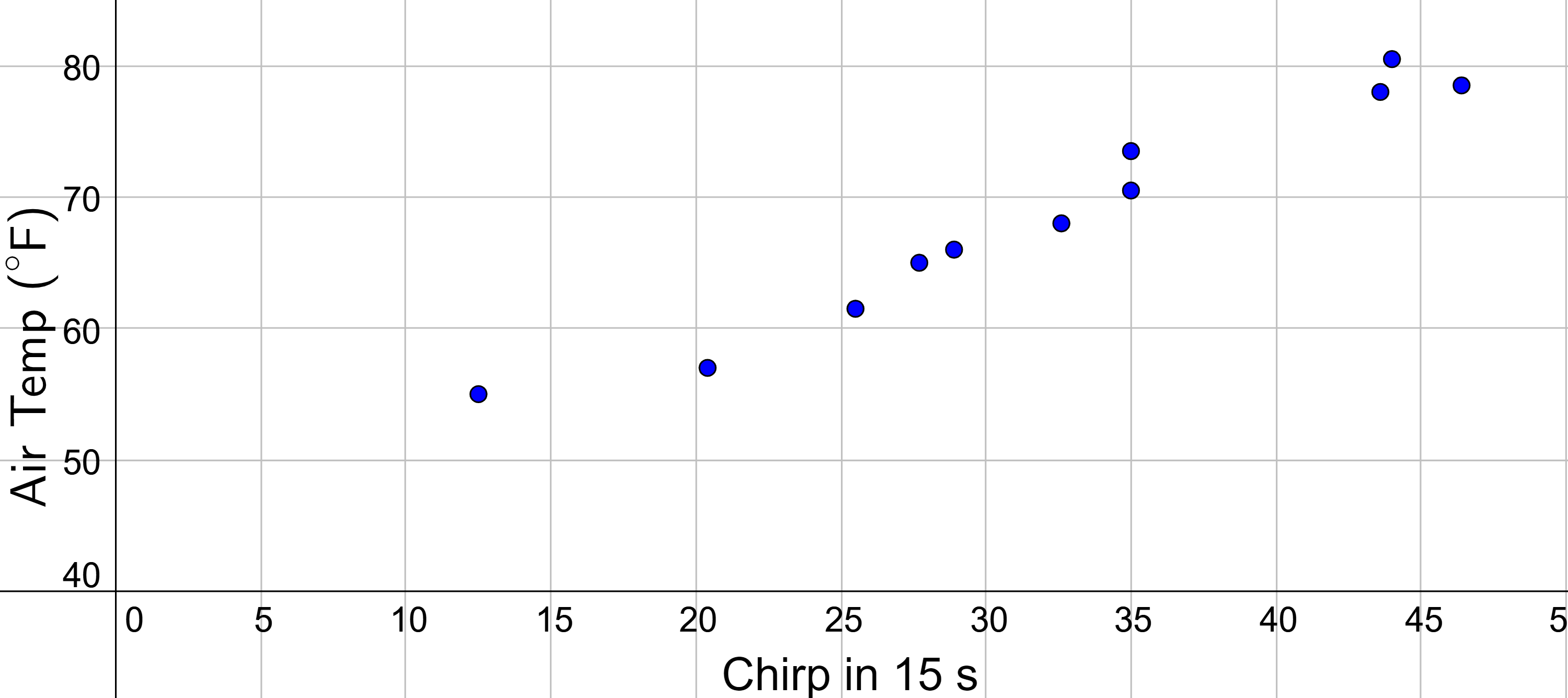
Physicist Amos Dolbear noticed that crickets chirped differently at different temperatures. He noticed that they chirped faster when it was hotter. So, he recorded how fast they chirped and the temperature. One way to analyze the data is to create a graph showing the number of chirps in 15 seconds versus the temperature. This is called creating a scatter plot.
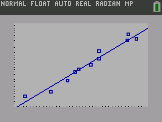
A scatter plot is a graph of points used to determine relationships between two sets of data. If the relationship is linear, then the points should lie along a straight line, and it could be modeled by a linear function. Figure 2 shows a scatter plot that seems to have a linear relationship.
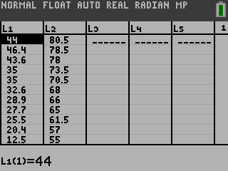
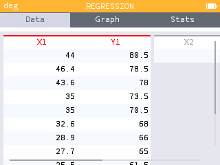
Table 1 shows the number of cricket chirps in 15 seconds, for several different air temperatures, in degrees Fahrenheit. Plot this data and determine whether the data appears to be linearly related.
| Chirps | 44 | 46.4 | 43.6 | 35 | 35 | 32.6 | 28.9 | 27.7 | 25.5 | 20.4 | 12.5 |
|---|---|---|---|---|---|---|---|---|---|---|---|
| Temp | 80.5 | 78.5 | 78 | 73.5 | 70.5 | 68 | 66 | 65 | 61.5 | 57 | 55 |
Solution
Graph the points as in figure 3. The temperature increases as the number of chirps increases in an approximately linear fashion. Thus, there is likely a relationship between temperature and the number of chirps a cricket makes in 15 seconds.
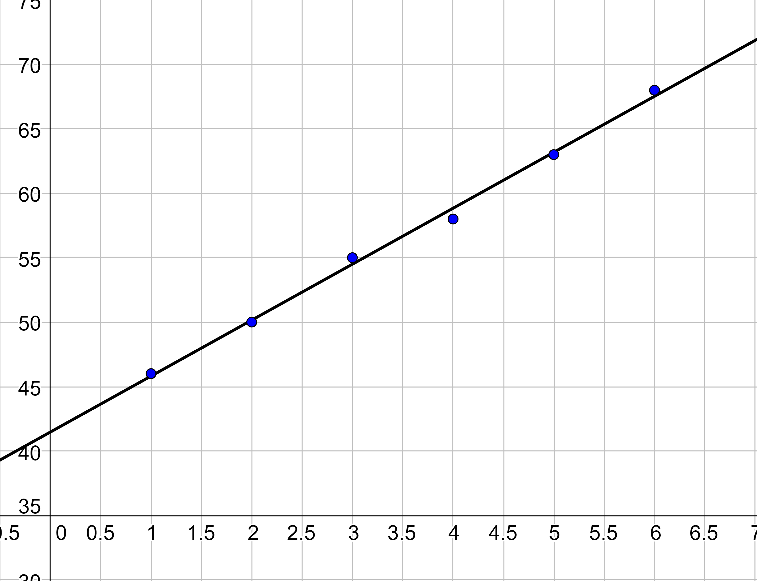
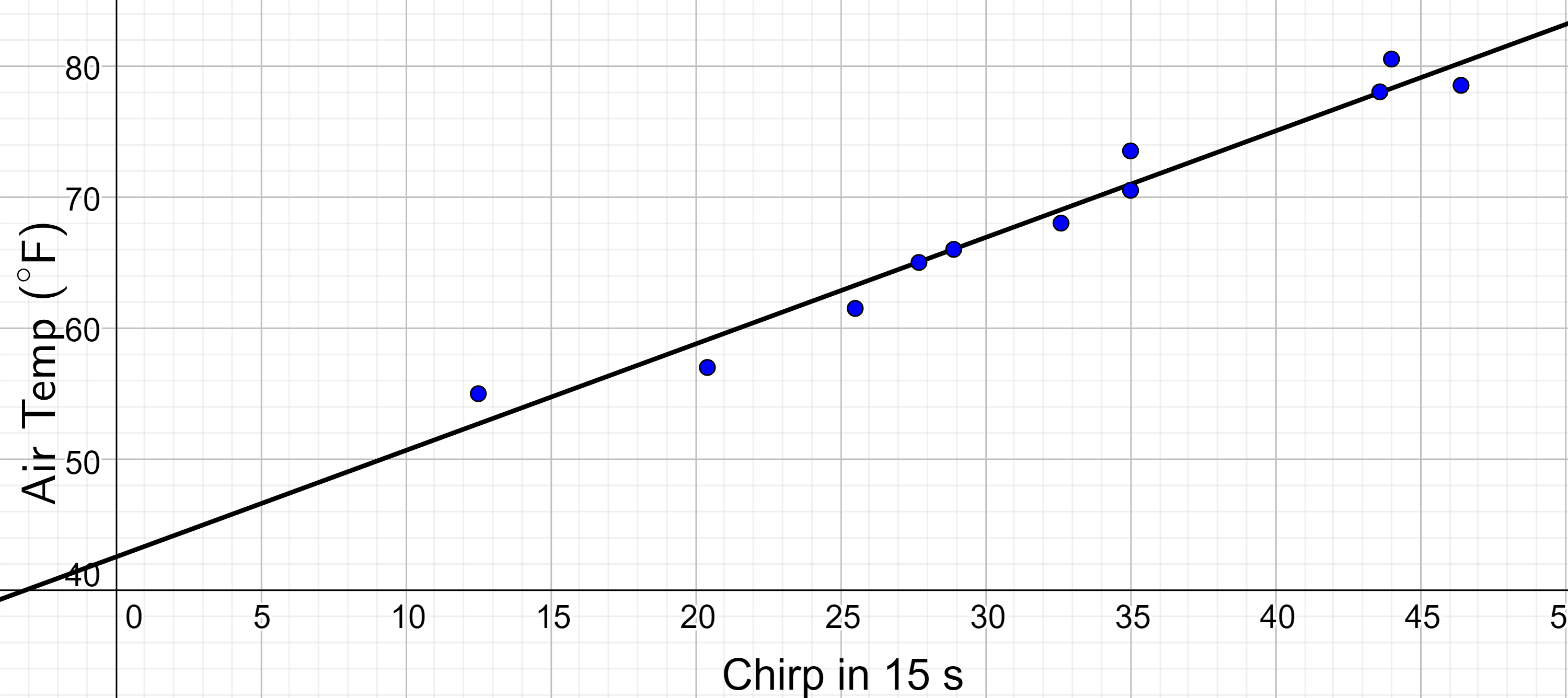
After identifying a linear relationship, it seems natural to ask, "What is the linear function?" One way to approximate the best-fitting line is to draw a best guess and then find the equation. When drawing the best guess, try to draw the line through the center of the points so that there are the same number of points above the line as below the line. The average distance from the points to the line needs to be made as small as possible.
Find a linear function that fits the data in table 1 by estimating the best fitting line.
Solution
Start by drawing a scatter plot of the data as was done in figure 3 which is duplicated here.
Draw a line that appears to go through the middle of all the data such as the line in figure 4.
Pick two points on the line. They do not have to be data point but could simply be places where the graph crosses the grid. The points should be far apart to reduce errors. The two red points in figure 5 will work well. Notice the point (9, 50) is not one of the original data points, but was read from the graph instead.
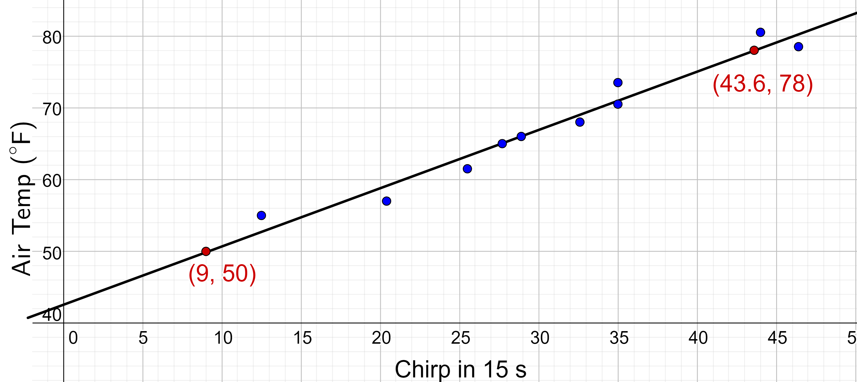
Find the slope between the two points, (9, 50) and (43.6, 78).
$$ slope = \frac{y_2 - y_1}{x_2 - x_1} $$
$$ m = \frac{78 - 50}{43.6 - 9} $$
m ≈ 0.8092
Finish finding the equation of the line through the points. Maybe use point-slope form with the point (9, 50).
y − y1 = m(x − x1)
y − 50 = 0.8092(x − 9)
y − 50 = 0.8092x − 7.2828
y − 50 = 0.8092x − 7.2828
y = 0.8092x + 42.7172
Finish by naming the variables something to represent the quantities. Perhaps call the y-variable T for temperature and the x-variable c for chirps.
T = 0.81c + 42.7
This linear equation can then be used to approximate answers to various questions asked about the trend.
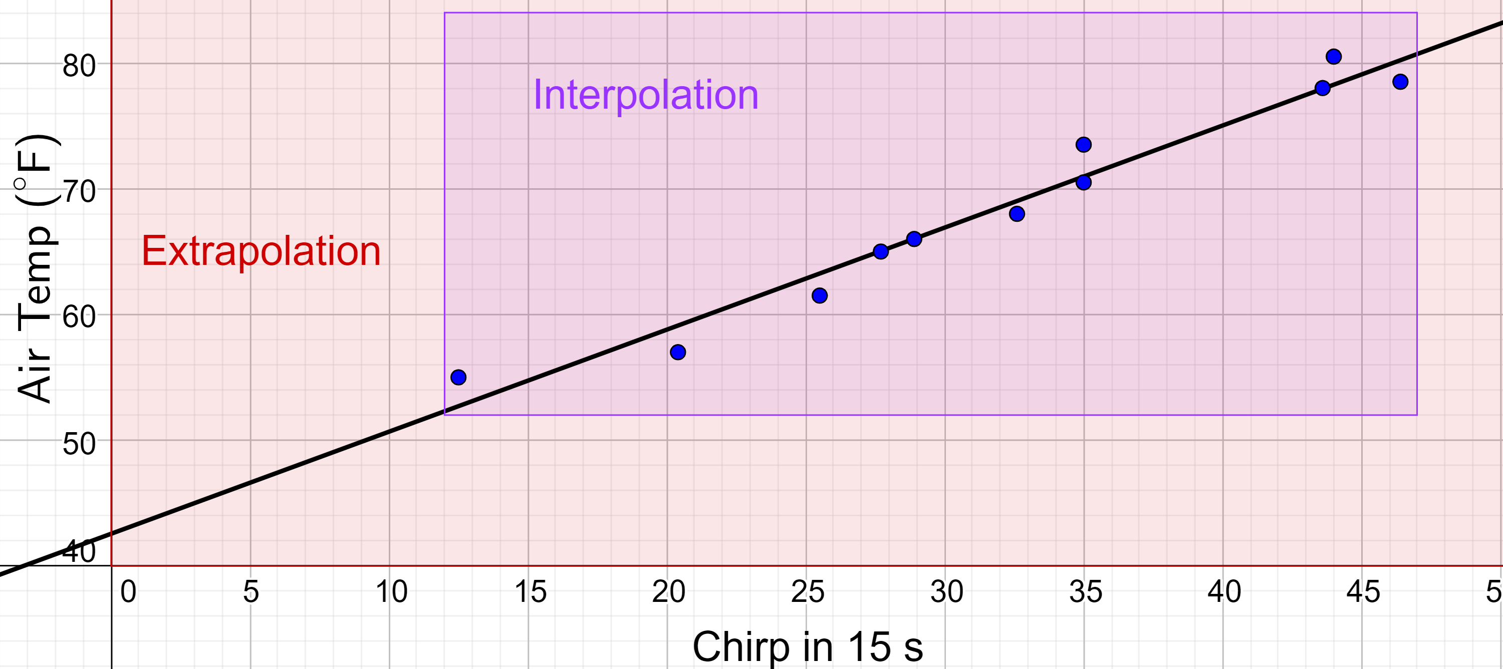
Notice the data points did not all fall perfectly on the best-fitting line. The equation is simply the best guess for how the relationship will be when it is not on one of the data points. Interpolation and extrapolation are used to make predictions based on the best-fitting line. Interpolation is predicting a value inside the domain and range of the data. Extrapolation is predicting a value outside of the domain and range of the data.
Figure 6 compares the two processes for the cricket-chirp data from Example 2. Interpolation occurs if the model is used to predict the temperature when the values for chirps are between 12.5 and 46.7. Extrapolation would occur if we used our model to predict temperature when the values for chirps are less than 12.5 or greater than 46.7.
There is a difference between making predictions inside the domain and range of values for which we have data and outside that domain and range. Interpolation is probably nearly correct because it is surrounded by other data. Extrapolation, or predicting a value outside of the domain and range has its limitations. The farther the extrapolation is from the data, the more likely the model no longer applies. This is sometimes called model breakdown. For example, using a few years of data to predict what happened millions of years ago, or even thousands of years in the future may give results that do not apply due to model breakdown. Extrapolation provides a guess but cannot provide a certainty.
Methods of making predictions and analyzing data.
Use the cricket data from to answer the following questions:
Solution
The number of chirps in the data provided varied from 12.5 to 46.7. A prediction at 30 chirps per 15 seconds is inside the domain of the data, so would be interpolation. Using the model:
T = 0.81c + 42.7
T = 0.81(30) + 42.7
T ≈ 67.0 °F
This is within the data, so this value seems reasonable.
The temperature values varied from 55 to 80.5. Predicting the number of chirps at 43 degrees is extrapolation because 43 is outside the range of the data. Using the model:
T = 0.81c + 42.7
43 = 0.81c + 42.7
0.3 = 0.81c
0.37 = c
The model predicts the crickets would chirp 0.37 times in 15 seconds. While this might be possible, there is no reason to believe the model is valid outside the domain and range. In fact, it has been observed that generally crickets stop chirping altogether below around 50 degrees.
According to the cricket-chirp data from example 2, what temperature can we predict it is if we counted 25 chirps in 15 seconds? Is this interpolation or extrapolation?
Answer
≈ 63.0 °F; interpolation
While estimating a best-fitting line works reasonably well, there are better statistical techniques for minimizing the distances from line to the data points. One such technique is called least squares regression and can be computed by many graphing calculators, spreadsheet software, statistical software, and many web-based calculators. Least squares regression is one means to determine the best-fitting for the data. Least squares regression is often called linear regression.

The calculator will display the equation. To see the graph of the points and line, press s.
Note: Older TI graphing calculators do not have the screen in steps 6 and 7. After selecting the LinReg(ax+b), the screen just shows LinReg(ax+b). Press Í again to see the result. To see the graph, enter the equation into the o screen and press s.
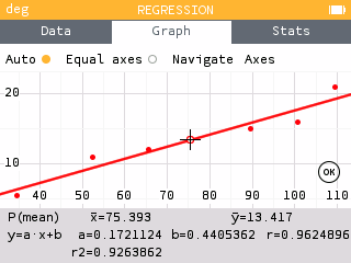
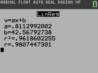
Find the least squares regression line using the cricket-chirp data in Table 1.
On a TI-84 graphing calculator
Note: To see the graph, enter Y1 for Store RegEQ: before pressing Calculate. Y1 is found in ½ ~ Y-VARS † Function… † Y1

T(c) = 0.811c + 42.57
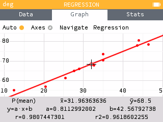
The graph of the scatter plot with the least squares regression line is shown in figure 12.
On a NumWorks graphing calculator

T(c) = 0.811c + 42.57
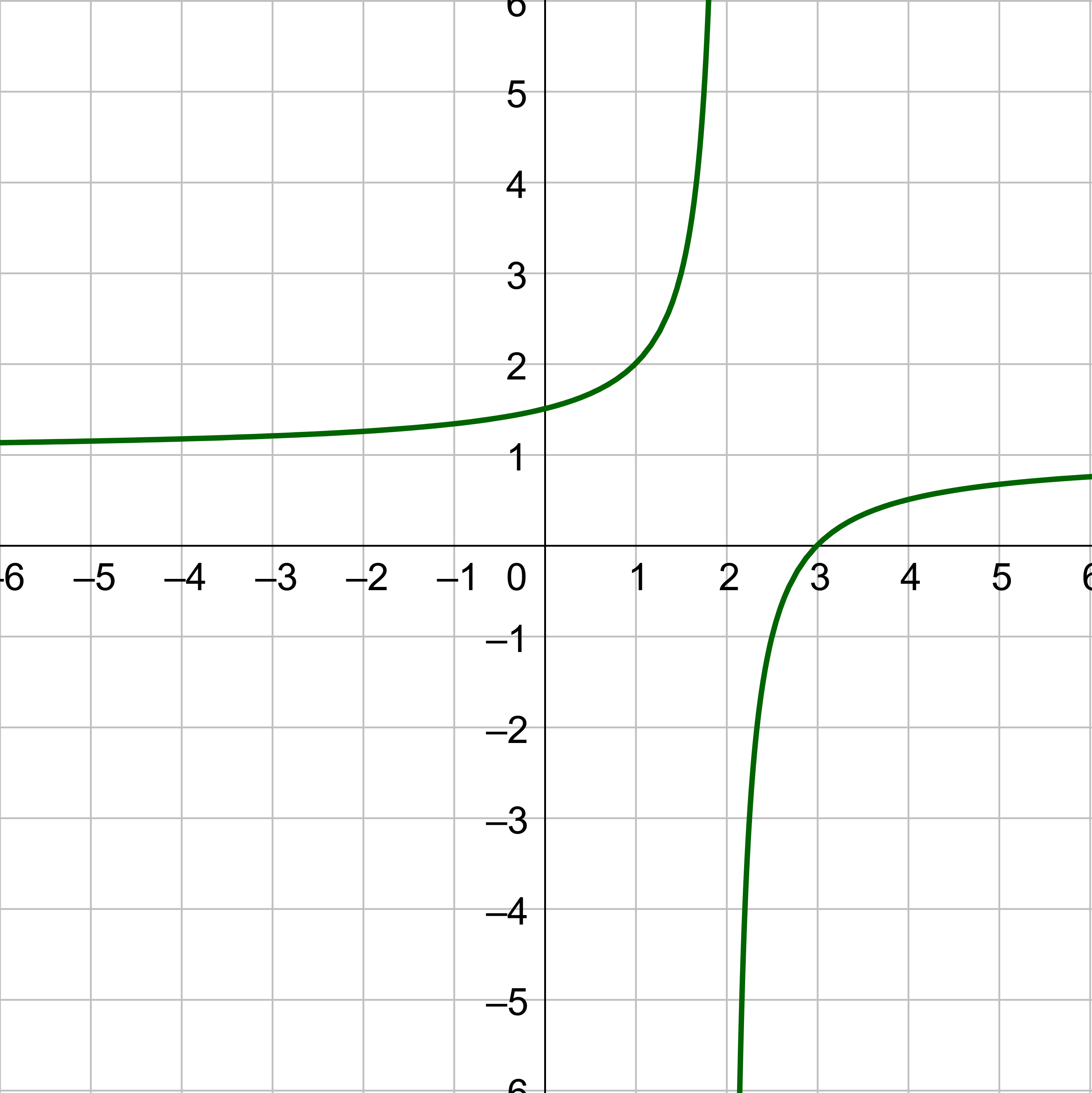
Some data such as the cricket-chirp model exhibit strong linear trends, but other data, like the height of a ball thrown in the air are nonlinear. Most calculators and computer software can also provide the correlation coefficient, r, which is a measure of how closely the line fits the data. Some graphing calculators require the user to use a “diagnostic on” selection to find the correlation coefficient. The correlation coefficient provides an easy way to get an idea of how close to a line the data falls. If r is very near 1 or −1, then the data is very linear; if r is near 0, then the data is not linear. However, the correlation coefficient should only be used on data that looks linear because some symmetric nonlinear data sets can have r = 1.
To get a sense for the relationship between the value of r and the graph of the data, figure 12 shows some large data sets with their correlation coefficients.
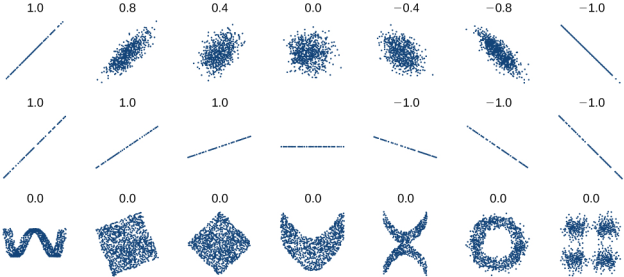
The correlation coefficient is a value, r, between –1 and 1.
Calculate the correlation coefficient for cricket-chirp data in table 1.
Solution
Because the data appear to follow a linear pattern, we can use a calculator to calculate r. Enter the inputs and corresponding outputs and select the Linear Regression. The calculator will also provide you with the correlation coefficient, r= 0.9808. This value is very close to 1, which suggests a strong increasing linear relationship.
Note: For some calculators, the Diagnostics must be turned “on” in order to get the correlation coefficient when linear regression is performed: For TI graphing calculators try z or N and scroll to DIAGNOSTICSON.
Some relationships depend only on one quantity, such as sales commissions. An employee who earns their pay by commission is given a percentage of the amount of sales he or she made. For example, Sally sells houses and earns 2% commission. If she sells a $250,000, then she earns 2% of $250,000 or (0.02)($250000) = $5000. Sally's earnings functions could be e = 0.02s where s is her sales. As her sales increase, her earnings also increase. This type of relationship, y = ax, is direct variation. Other types of variations are given in the box below.
In all cases, a is the constant of variation.
y varies directly with the square of x. If y = 32 when x = 5, find the equation relating x and y. Then find y when x is 6.
Solution
Because the problem uses x and y, the input is x2 and the output is y. The problem states that this is direct variation. Write the general equation of direct variation.
y = ax2
Fill in the given value of x and y.
32 = a(52)
Solve for the constant a.
32 = a(25)
$$ a = \frac{32}{25} $$
Now use the constant to write an equation that represents this relationship.
$$ y = \frac{32}{25}x^2 $$
Substitute x = 6 and solve for y.
$$ y = \frac{32}{25}(6^2) $$
$$ y = \frac{1152}{25} $$
y varies directly with the cube of x. If y = 24 when x = 3, find the equation relating x and y. Then find y when x is 5.
Answer
\(y = \frac{8}{9}x^3\); \(\frac{1000}{9}\)
In electricity, the current, I, of a circuit varies inversely with the resistance, R. In this particular circuit, the current is 0.0015 A when the resistance is 1000 Ω. Write a function relating the current and the resistance of the circuit.
Solution
The input is the resistance, R, and the output is the current, I. This is usually distinguishable because the current came first in the problem sentence. The problem states it is an inverse variation. Write the general equation for inverse variation.
$$ y = \frac{a}{x} $$
Because it is the input, replace the x with the resistance, R. Also, replace the output y with the current, I.
$$ I = \frac{a}{R} $$
Fill in the given values and solve for a.
$$ 0.0015 = \frac{a}{1000} $$
1.5 = a
Substitute a into the model.
$$ I = \frac{1.5}{R} $$
A quantity y varies inversely with the square of x. If y = 25 when x = 4, find the equation relating x and y. Then find y when x is 2.
Solution
The input is x2 and the output is y. Write the general equation for inverse variation.
$$ y = \frac{a}{x^2} $$
Fill in the given values and solve for a.
$$ 25 = \frac{a}{4^2} $$
400 = a
Substitute a into the model.
$$ y = \frac{400}{x^2} $$
Now fill in x = 2 and find y.
$$ y = \frac{400}{2^2} $$
y = 100
A quantity y varies inversely with the cube of x. If y = 4 when x = 3, find the equation relating x and y. Then find y when x is 2.
Answer
\(y = \frac{108}{x^3}\); \(\frac{27}{2}\)
A quantity x varies jointly with the square of y cube root of z. If x = 20 when y = 2 and z = 8, find the equation relating the quantities. Then find x when y = 1 and z = 27.
Solution
The output is x because it comes first in the sentence. The inputs are y2 and \(\sqrt[3]{z}\). Write the equation as suggested by the sentence. The word "varies" indicates "= a".
$$ x = ay^2 \sqrt[3]{z} $$
Fill in the given values and solve for a.
$$ 20 = a(2^2)\sqrt[3]{8} $$
$$ 20 = a(8) $$
$$ \frac{5}{2} = a $$
Substitute a into the model.
$$ x = \frac{5}{2}y^2\sqrt[3]{z} $$
Now fill in y = 1 and z = 27 and find x.
$$ x = \frac{5}{2}(1^2)\sqrt[3]{27} $$
$$ x = \frac{15}{2} $$
x varies directly with the square of y and inversely with z. If x = 40 when y = 4 and z = 2, find the equation relating the quantities. Then find x when y = 10 and z = 25.
Answer
\(x = \frac{5y^2}{z}\); 20
Methods of making predictions and analyzing data.
The calculator will display the equation. To see the graph of the points and line, press s.
Note: Older TI graphing calculators do not have the screen in steps 6 and 7. After selecting the LinReg(ax+b), the screen just shows "LinReg(ax+b)". Press Í again to see the result. To see the graph, enter the equation into the o screen and press s.
The correlation coefficient is a value, r, between –1 and 1.
In all cases, a is the constant of variation.
Helpful videos about this lesson.
| 1 | 2 | 3 | 4 | 5 | 6 |
| 46 | 50 | 55 | 58 | 63 | 68 |
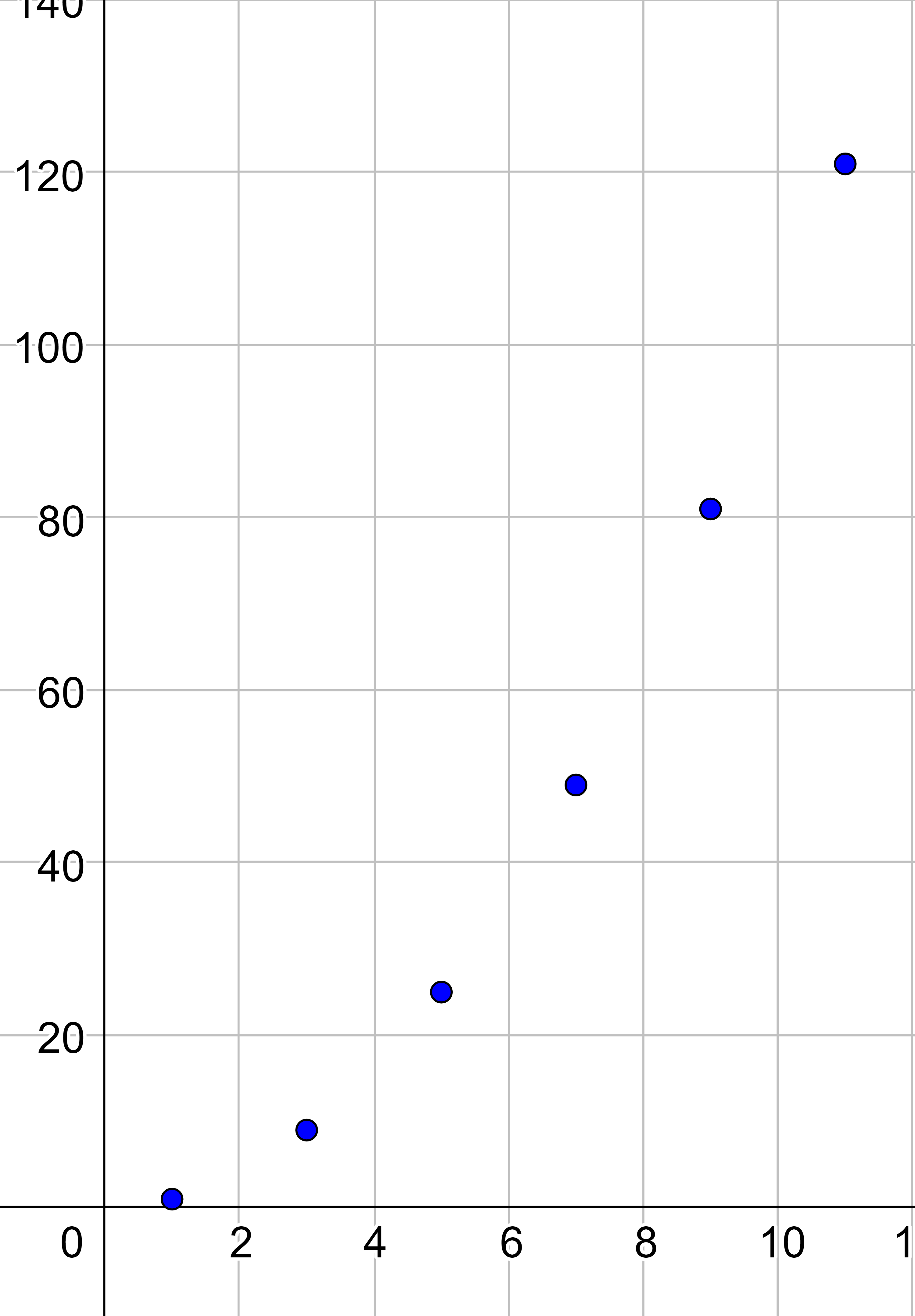
| 1 | 3 | 5 | 7 | 9 | 11 |
| 1 | 9 | 25 | 49 | 81 | 121 |
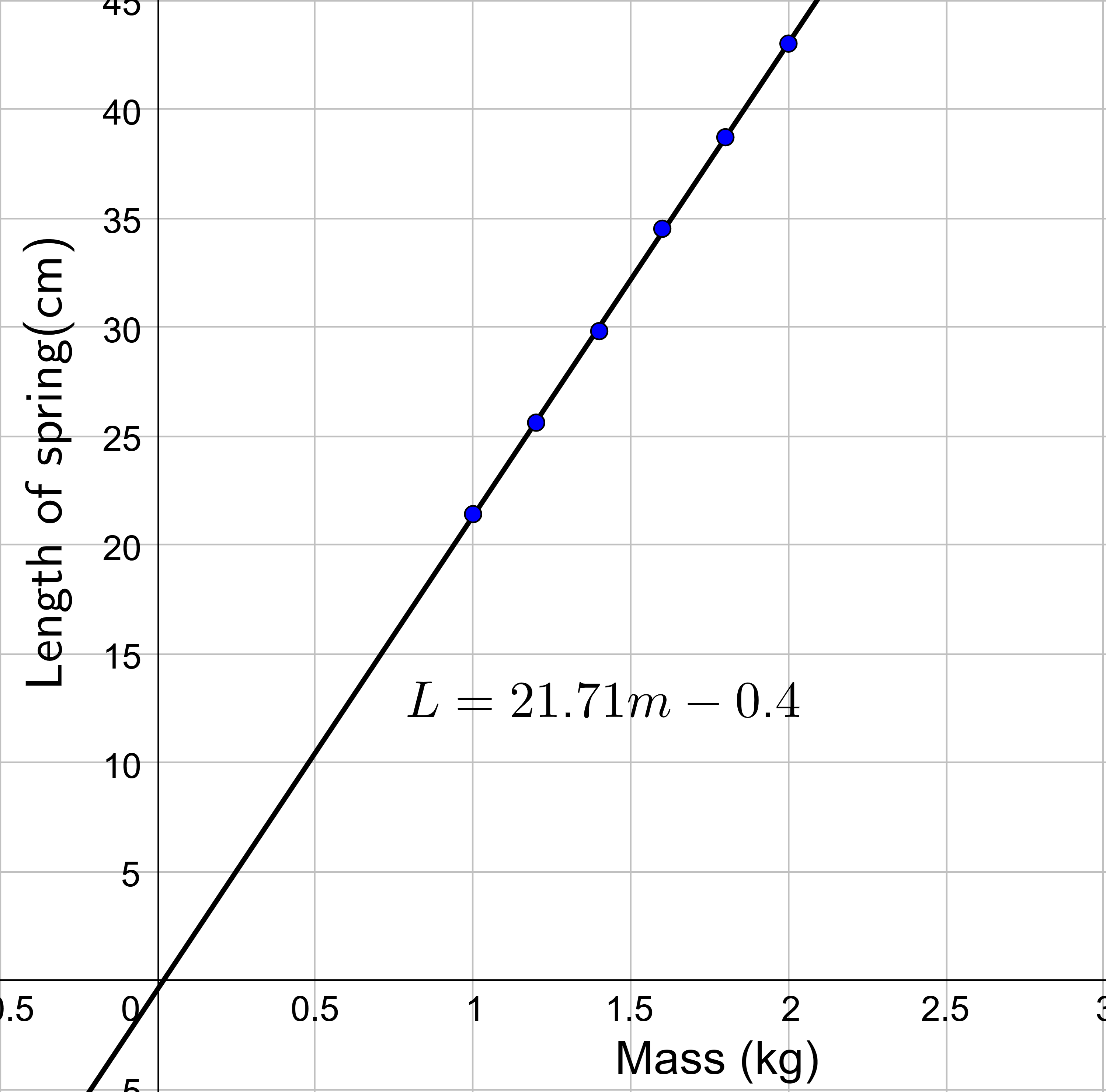
| Mass (kg) | 1.0 | 1.2 | 1.4 | 1.6 | 1.8 | 2.0 |
|---|---|---|---|---|---|---|
| Length (cm) | 21.4 | 25.6 | 29.8 | 34.5 | 38.7 | 43.0 |
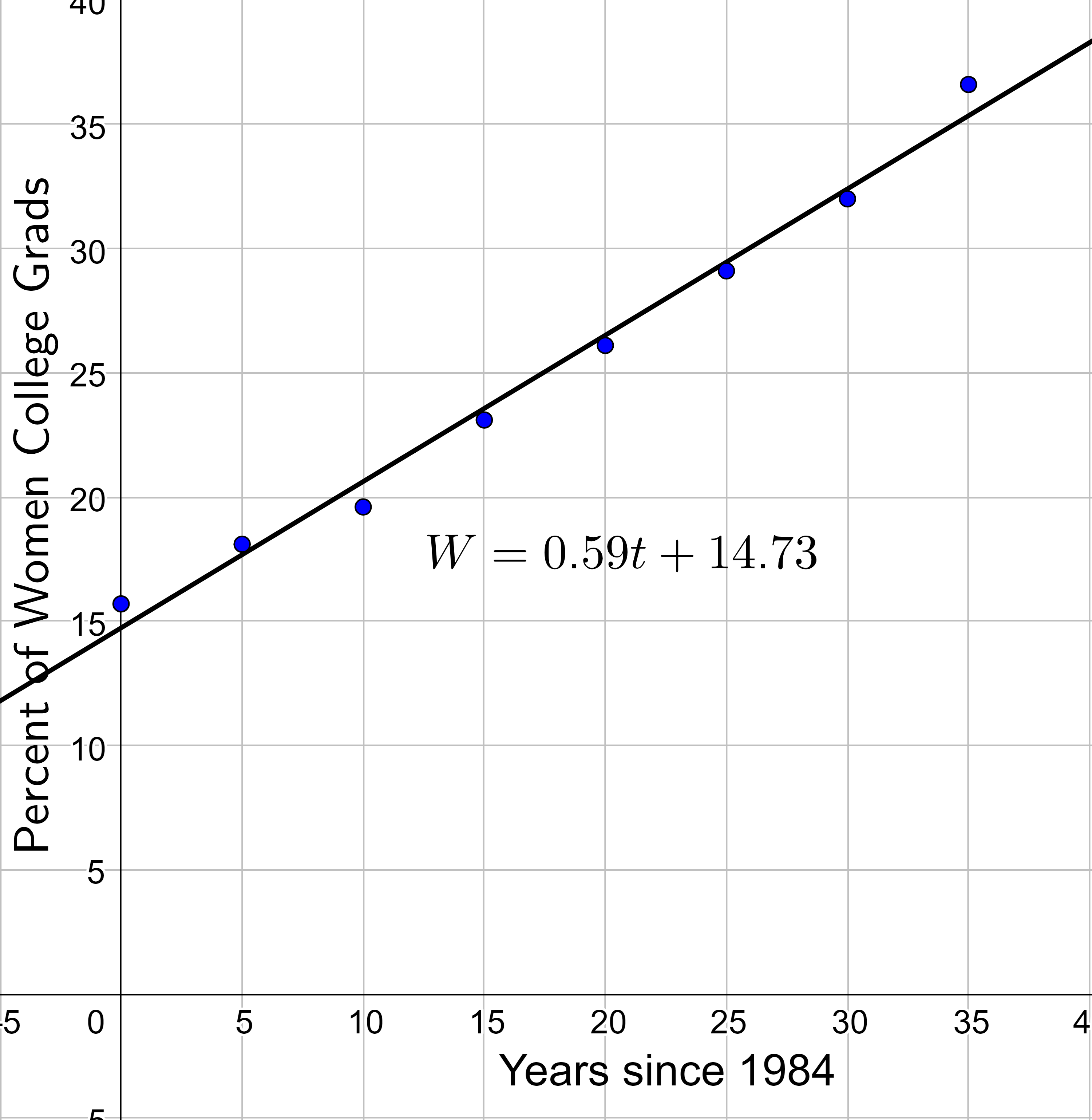
| Year | 1984 | 1989 | 1994 | 1999 | 2004 | 2009 | 2014 | 2019 |
|---|---|---|---|---|---|---|---|---|
| Percent Graduates | 15.7 | 18.1 | 19.6 | 23.1 | 26.1 | 29.1 | 32.0 | 36.6 |
| x | 2 | 15 | 26 | 30 | 55 |
|---|---|---|---|---|---|
| y | 0 | 19 | 36 | 42 | 79 |
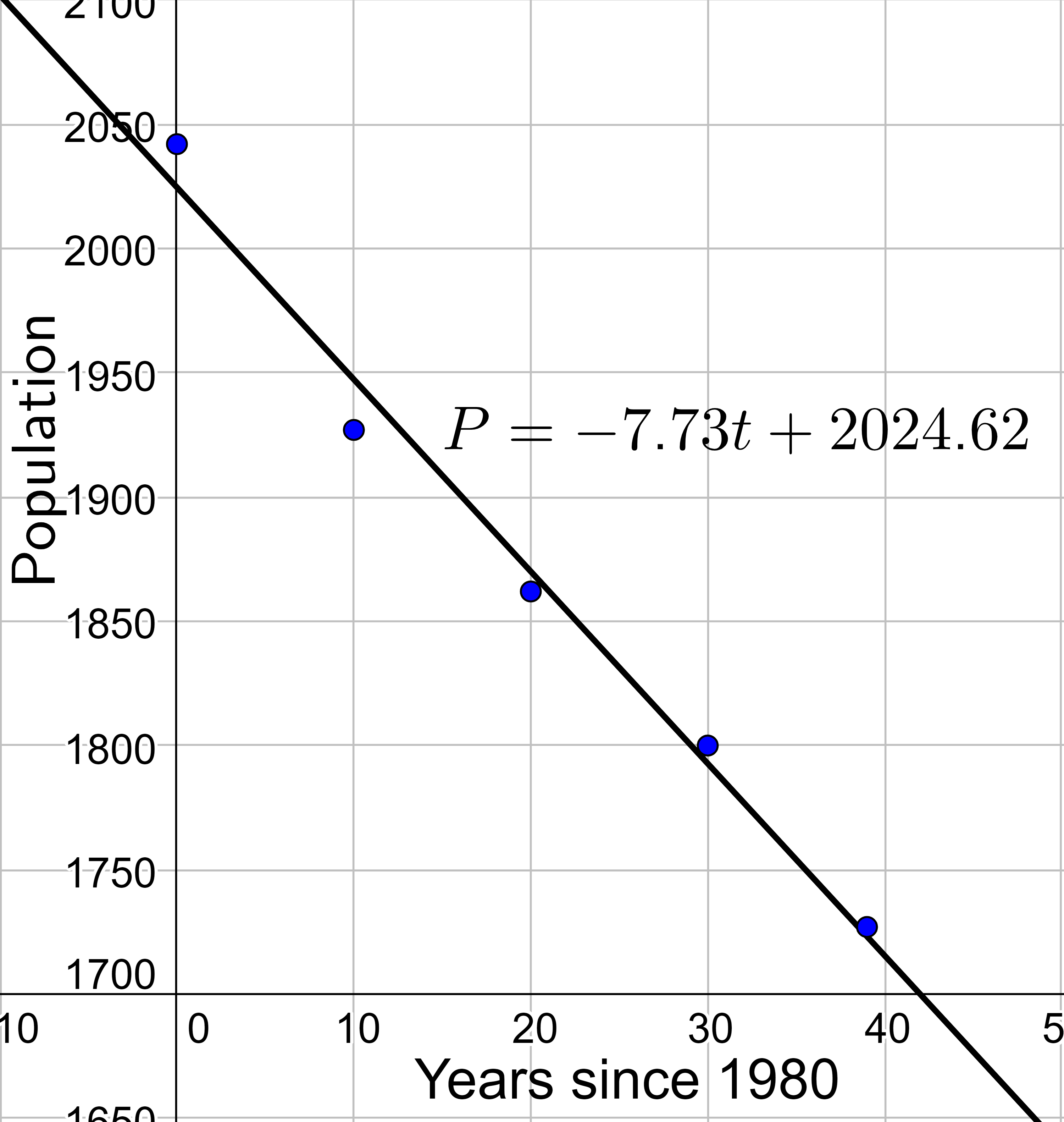
| Year | 1980 | 1990 | 2000 | 2010 | 2019 |
|---|---|---|---|---|---|
| Population | 2042 | 1927 | 1862 | 1800 | 1727 |